Cell Simulations with the Marching Cubes Algorithm
By Lisa Lau and Tyler Wolf Leonhardt
1 - Abstract
The marching cubes algorithm is an algorithm which allows a mesh to be created from a scalar field [1]. In other words, the algorithm takes a 3-dimensional array of points with certain intensities and creates a mesh which represent a volume of neighbor points above a certain intensity threshold. This algorithm can be used to create many different types of procedurally generated meshes. One of the procedurally generated meshes that this algorithm can create is called a meatball. Metaballs are spherical objects which modify the geometry of other metaballs, sometimes even to the point of fusing, when they are close to each other [2]. The geometry created by two metaballs traveling away from each other is roughly similar to that of a cell during mitosis. In the following report we provide information about our implementation of the marching cubes algorithm and describe how we used it to generate a cell-mitosis animation.
2 - The Algorithm
On its own the marching cubes algorithm requires a large amount of code. The implementation of the cell-mitosis was originally implemented using open-source code found online [3]. This algorithm was much too slow for our use and had to be completely rewritten. For simplicity we divided the algorithm across a collection of classes. Classes of importance are described in the subsection, below and the computation itself is described in the following subsection.
2.1 - Classes
2.1.1 - MarchingCubesEnvironment
The environment which the generated mesh can live in. This class allows the number of cubes in the environment to be specified along each axis. Increasing the number of cubes increases the quality of the mesh but the mesh also takes longer to generate. If part of the mesh leaves the bounds specified by the environment it will no longer be visible. After the environment is created, the cubes within it can be indexed as though they were members of an array.
2.1.2 - MarchingEntity
An entity within the environment. This entity gives the points in the environment their intensities. Each entity can generate intensities however it wishes.
2.1.2 - MarchingMetaball
A marching entity which generates intensities using the following equation:

The square magnitude was used so that a square root did not have to be taken for every point. This computation would have been prohibitively expensive. Additionally, the elimination of the floating point division would also have provided a much more computationally efficient equation.
2.1.4 - MarchingCube
A cube within the environment with local space coordinates between -0.5 and +0.5 in each direction (X, Y, Z). It consists of 8 points and 12 edges.
2.1.5 - MarchingEdge
An edge within the environment. It consists of 2 points.
2.1.6 - MarchingPoint
A point within the environment.
2.1.7 - EdgeIndex
The 0-11 index of an edge in a marching cube.
2.1.8 - PointIndex
The 0-7 index of a point in a marching cube.
2.1.9 - EdgeFlags
Flags indicating which edges will contain a vertex if the cube were drawn.
2.1.10 - PointFlags
Flags indicating which points have an intensity above the threshold. These flags are all adjacent numbers within the range 0-255 so they can be used to index an array.
2.1.11 - PointFlagsToEdgeConverter
Converts point flags to edge flags or to a list of edge indices using tables generated from a utility.
2.2 - Computation
The following procedure describes this particular implementation of the algorithm:
- Get the set of entities which we wish to create a mesh for.
- Remove one entity from the set and determine where its centroid is located in the local-space of the marching cubes environment.
- Convert the local-space coordinates to an index into the cube-lattice. Clamp the coordinates if the entity is outside of the bounds.
- Search all cubes starting from our index along the Z-axis towards the closest edge of the environment applying intensities to their points as we go, stop when we find a cube at the surface of the mesh, the edge of the environment, or a cube that has already been searched.
- If we found a new cube at the surface of the mesh search all of the neighboring cubes and repeat this step.
The following procedure describes how a cube is searched:
- Calculate the intensity at each point in the cube.
- Obtain a set of point flags indicating which points are on.
- Obtain a set of edge flags from the point flags using the point flags to edge converter.
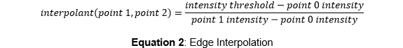
- Interpolate new points along each of these edges using their constituent points and the point intensities and assign an index to each edge. Essentially linearly interpolate the two points and use the result of the following equation as the interpolant:
- Add the new interpolated points to a list of vertexes we will draw.
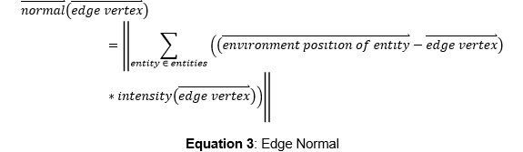
- Calculate the normal of each of the edges we just added using the following equation:
- Add the new normal to a list of the normal of each vertex we will draw. They should be added in the same order that the vertices were added in.
- Obtain a set of indices from the point flags indicating the edges of the cube which will be used as triangles. Index the cube for these edges and add their indices to a list of triangle indices.
After all of the cubes are searched and the lists of vertices, normal and triangle indices are built the new mesh can be generated.
2.3 - Results
2.3.1 - Overall Simulation
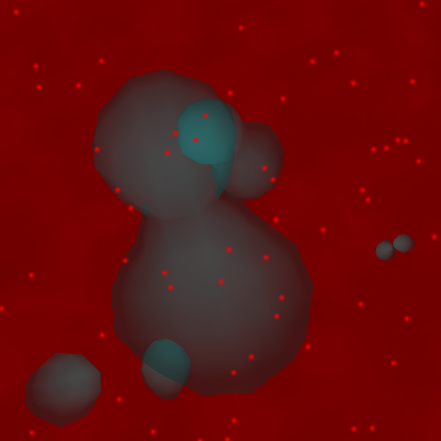
For the overall simulation 11 marching cubes environments were created and 8 metaballs were added to each environment. Each environment contained 15 cubes in each direction totaling 3,375 cells each or 37,125 total cells. The meshes of each environment were textured with a transparent texture and shaded with a transparent diffuse shader. The metaballs were clustered in groups of two within their environment so that they could be easily controlled. Two sets of the metaballs could be controlled using the up and down arrow keys on a standard keyboard: the up key would bring the balls apart and the down key would bring them together. The rest of the balls were controlled automatically using scripts. A skybox, light, music and particle effects were also provided for atmosphere. The simulation ran with an average framerate around 30 FPS on a test laptop. Figure 1, below, provides an example of what the scene looked like.
|
|
Figure 1: Overall Simulation
|
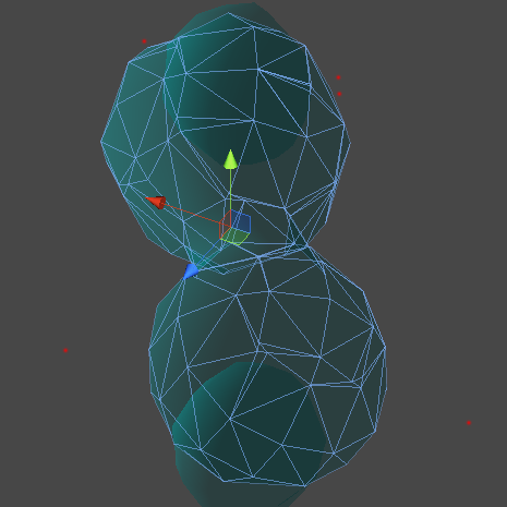
Figure 2, below provides an example of the vertices used to create the central cell.
|
|
Figure 2: Overall Central Cell Mesh
|
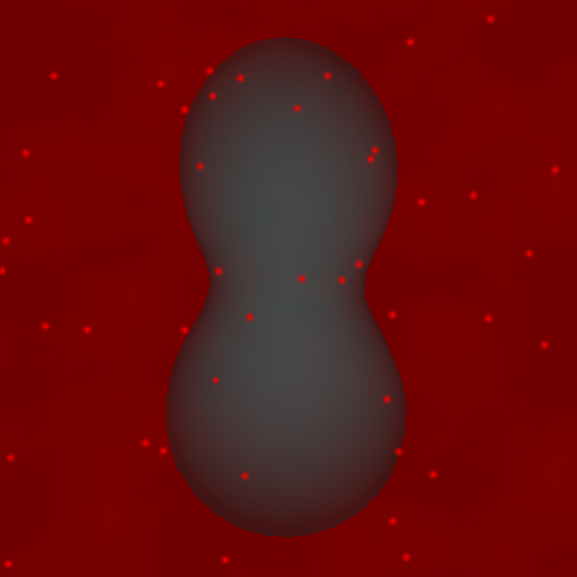
2.3.2 - Single Cell
For the single-cell simulation 1 marching cubes environments was created and 8 metaballs were added to the environment. The environment contained 60 cubes in each direction totaling 216,000 cells. The meshes of the environment were textured with a transparent texture and shaded with a transparent diffuse shader. The metaballs were clustered in two group within the environment so that they could be easily controlled. The two sets of the metaballs could be controlled using the up and down arrow keys on a standard keyboard: the up key would bring the balls apart and the down key would bring them together. A skybox, light, music and particle effects were also provided for atmosphere. The simulation ran with an average framerate around 30 FPS on a test laptop. Figure 3, below, provides an example of what the scene looked like.
|
|
Figure 3: Single Cell Simulation
|
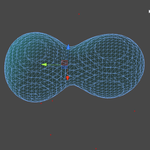
Figure 4, below provides an example of the vertices used to create the cell.
|
|
Figure 4: Single Cell Mesh
|
3 - References
4 - Additional Resources
The source code described within this document is available at https://github.com/Tyleo/cellzilla.
The application described within this document can be run using Unity Web Player at http://tyleo.github.io/cellzilla/app/cellzilla-single.html. This simulation demonstrates a single cell with 60 cubes along each row.
A video of the application running is available at http://tyleo.github.io/cellzilla/video/video.html